Examples

The following examples show how to solve common tasks using opda.

To dive deeper, checkout Usage or the API Reference.

Compare Models

Let’s compare two models while accounting for hyperparameter tuning effort. We could compare a new model against a baseline or perhaps against an ablation of some component. Either way, the comparison works pretty much the same.

Models with Similar Costs

If the models have similar costs (e.g., training compute), then compare their performance as a function of hyperparameter search iterations:

>>> from matplotlib import pyplot as plt
>>> import numpy as np
>>>
>>> from opda.nonparametric import EmpiricalDistribution
>>>
>>> generator = np.random.default_rng(0)  # Set the random seed.
>>> uniform = generator.uniform
>>>
>>> # Simulate results from random search.
>>> ys0 = uniform(0.70, 0.90, size=48)  # scores from model 0
>>> ys1 = uniform(0.75, 0.95, size=48)  # scores from model 1
>>>
>>> # Plot tuning curves and confidence bands for both models in one figure.
>>> fig, ax = plt.subplots()
>>> ns = np.linspace(1, 10, num=1_000)
>>> for name, ys in [("baseline", ys0), ("model", ys1)]:
...   # Construct the confidence bands.
...   dist_lo, dist_pt, dist_hi = EmpiricalDistribution.confidence_bands(
...     ys=ys,            # accuracy results from random search
...     confidence=0.80,  # confidence level
...     a=0.,             # (optional) lower bound on accuracy
...     b=1.,             # (optional) upper bound on accuracy
...   )
...   # Plot the tuning curve.
...   ax.plot(ns, dist_pt.quantile_tuning_curve(ns), label=name)
...   # Plot the confidence bands.
...   ax.fill_between(
...     ns,
...     dist_hi.quantile_tuning_curve(ns),
...     dist_lo.quantile_tuning_curve(ns),
...     alpha=0.275,
...     label="80% confidence",
...   )
...   # Format the plot.
...   ax.set_xlabel("search iterations")
...   ax.set_ylabel("accuracy")
...   ax.set_title("Model Comparison")
...   ax.legend(loc="lower right")
[<matplotlib...
>>> # plt.show() or fig.savefig(...)

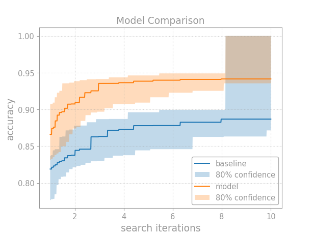
Breaking down this example, first we construct confidence bands for each model’s CDF using confidence_bands():

>>> for name, ys in [("baseline", ys0), ("model", ys1)]:
...   # Construct the confidence bands.
...   dist_lo, dist_pt, dist_hi = EmpiricalDistribution.confidence_bands(
...     ys=ys,            # accuracy results from random search
...     confidence=0.80,  # confidence level
...     a=0.,             # (optional) lower bound on accuracy
...     b=1.,             # (optional) upper bound on accuracy
...   )

Then, we compute the tuning curves via the quantile_tuning_curve() method. The lower CDF band gives the upper tuning curve band, and the upper CDF band gives the lower tuning curve band. In this way, you can plot the tuning curve with confidence bands:

...   # Plot the tuning curve.
...   ax.plot(ns, dist_pt.quantile_tuning_curve(ns), label=name)
...   # Plot the confidence bands.
...   ax.fill_between(
...     ns,
...     dist_hi.quantile_tuning_curve(ns),
...     dist_lo.quantile_tuning_curve(ns),
...     alpha=0.275,
...     label="80% confidence",
...   )

The rest just makes the plot look pretty, then shows it or saves it to disk.

Models with Different Costs

When models have different costs, it’s more difficult to make a comparison. Use your judgment and tailor the analysis to the situation.

One general approach is: first rescale the models so they have similar inference cost, then adjust the tuning curves to match the training cost. To adjust the tuning curves, just multiply the search iterations by their average cost (e.g., in FLOPs, GPU hours, dollars, and so on).

Let’s revisit the previous example. This time, assume the models have similar sizes; however, while the baseline trains for 1 epoch, the new model trains for 1 to 5:

>>> # Compute the average cost per training run.
>>> avg_epochs0 = 1                         # train model 0 for 1 epoch
>>> avg_epochs1 = np.mean([1, 2, 3, 4, 5])  # train model 1 for 1-5 epochs
>>>
>>> # Plot tuning curves and confidence bands for both models in one figure.
>>> fig, ax = plt.subplots()
>>> ns = np.linspace(1, 30, num=1_000)
>>> for name, avg_epochs, ys in [
...   ("baseline", avg_epochs0, ys0),
...   (   "model", avg_epochs1, ys1),
... ]:
...   # Construct the confidence bands.
...   dist_lo, dist_pt, dist_hi = EmpiricalDistribution.confidence_bands(
...     ys=ys,            # accuracy results from random search
...     confidence=0.80,  # confidence level
...     a=0.,             # (optional) lower bound on accuracy
...     b=1.,             # (optional) upper bound on accuracy
...   )
...   # Plot the tuning curve.
...   ax.plot(
...     avg_epochs * ns,
...     dist_pt.quantile_tuning_curve(ns),
...     label=name,
...   )
...   # Plot the confidence bands.
...   ax.fill_between(
...     avg_epochs * ns,
...     dist_hi.quantile_tuning_curve(ns),
...     dist_lo.quantile_tuning_curve(ns),
...     alpha=0.275,
...     label="80% confidence",
...   )
...   # Format the plot.
...   ax.set_xlim(1, 30)
...   ax.set_xlabel("total training epochs")
...   ax.set_ylabel("accuracy")
...   ax.set_title("Model Comparison")
...   ax.legend(loc="lower right")
[<matplotlib...
>>> # plt.show() or fig.savefig(...)

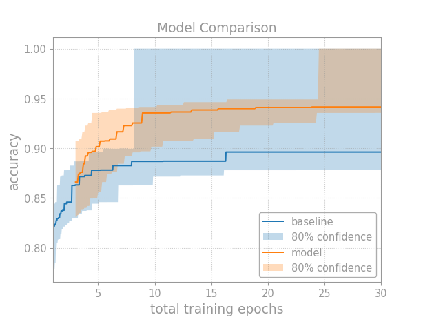
The main difference is that we multiply the number of search iterations by their average cost. First, we compute the average cost per training run:

>>> # Compute the average cost per training run.
>>> avg_epochs0 = 1                         # train model 0 for 1 epoch
>>> avg_epochs1 = np.mean([1, 2, 3, 4, 5])  # train model 1 for 1-5 epochs

While the baseline trains for 1 epoch, the new model trains for 1 to 5 at random. In general, pick the cost measure and way to compute the average that’s most appropriate for your problem. Here, we use total training epochs and the formula for a mean. If we compared two optimizers instead, we might use FLOPs and either calculate the average theoretically[1] or estimate it empirically based on the results from our random search—but, be careful! Since we won’t account for uncertainty in the average cost, you must use a high quality estimate.

When you plot the tuning curve, multiply the search iterations by the average cost per training run:

...   # Plot the tuning curve.
...   ax.plot(
...     avg_epochs * ns,
...     dist_pt.quantile_tuning_curve(ns),
...     label=name,
...   )
...   # Plot the confidence bands.
...   ax.fill_between(
...     avg_epochs * ns,
...     dist_hi.quantile_tuning_curve(ns),
...     dist_lo.quantile_tuning_curve(ns),
...     alpha=0.275,
...     label="80% confidence",
...   )

Note that we only multiply the x values by the average cost. The quantile_tuning_curve() method still expects the number of search iterations as input.

And that’s it! We now have a fair comparison between models based on our tuning budget.

To learn more, checkout EmpiricalDistribution in the reference documentation or get interactive help in a Python REPL by running help(EmpiricalDistribution).

Analyze a Hyperparameter

Let’s determine whether a specific hyperparameter is important to tune and then dig into how it affects performance. We might, for example, do this after comparing a model against a baseline in order to understand the new model or provide advice on tuning its hyperparameters.

Hyperparameter Importance

Imagine we’re pretraining a language model. We’re interested in the weight decay. First, let’s ask: how important is this hyperparameter? Weerts et al. (2020) give a practical and intuitive definition of hyperparameter importance in terms of tuning risk: the difference in test performance between tuning the hyperparameter and leaving it at the default value. We’ll operationalize this idea by comparing the tuning curve from when we do tune the hyperparameter to the one where we don’t:

>>> from matplotlib import pyplot as plt
>>> import numpy as np
>>>
>>> from opda.nonparametric import EmpiricalDistribution
>>>
>>> generator = np.random.default_rng(0)  # Set the random seed.
>>> normal, uniform = generator.normal, generator.uniform
>>>
>>> # Design the experiment.
>>> n = 48            # Decide the number of search iterations.
>>> search_space = {  # Define the search space.
...   "learning_rate": {"bounds": [1e-5, 1e-1], "default": 1e-3},
...   "weight_decay" : {"bounds": [1e-6, 1e-2], "default": 1e-4},
... }
>>>
>>> # Run random search on the hyperparameters.
>>> def pretrain(learning_rate, weight_decay):
...   xentropy = 1. \
...     + (np.log10(learning_rate) - -2)**2 / 2 \
...     + (np.log10( weight_decay) - -6)**2 / 7
...   return xentropy + normal(0, 0.1, size=xentropy.size)
>>>
>>> ys_default = pretrain(  # Set weight decay to default.
...   learning_rate=np.exp(uniform(np.log(1e-5), np.log(1e-1), size=n)),
...   weight_decay=1e-4,
... )
>>> ys_tuned = pretrain(    # Tune weight decay.
...   learning_rate=np.exp(uniform(np.log(1e-5), np.log(1e-1), size=n)),
...   weight_decay =np.exp(uniform(np.log(1e-6), np.log(1e-2), size=n)),
... )
>>>
>>> # Plot tuning curves and confidence bands for both conditions.
>>> fig, ax = plt.subplots()
>>> ns = np.linspace(1, 10, num=1_000)
>>> conditions = [
...   (      "default (1e-4)", ys_default),
...   ("tuned (1e-6 to 1e-2)",   ys_tuned),
... ]
>>> for name, ys in conditions:
...   # Construct the confidence bands.
...   dist_lo, dist_pt, dist_hi = EmpiricalDistribution.confidence_bands(
...     ys=ys,            # cross-entropy results from random search
...     confidence=0.80,  # confidence level
...     a=0.,             # (optional) lower bound on cross-entropy
...     b=np.inf,         # (optional) upper bound on cross-entropy
...   )
...   # Plot the tuning curve.
...   ax.plot(
...     ns,
...     dist_pt.quantile_tuning_curve(ns, minimize=True),
...     label=name,
...   )
...   # Plot the confidence bands.
...   ax.fill_between(
...     ns,
...     dist_hi.quantile_tuning_curve(ns, minimize=True),
...     dist_lo.quantile_tuning_curve(ns, minimize=True),
...     alpha=0.275,
...     label="80% confidence",
...   )
...   # Format the plot.
...   ax.set_xlabel("search iterations")
...   ax.set_ylabel("cross-entropy")
...   ax.set_title("Weight Decay Importance")
...   ax.legend(loc="upper right")
[<matplotlib...
>>> # plt.show() or fig.savefig(...)

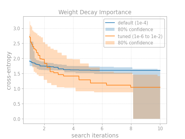
Breaking down this example, first we run a (hypothetical) random search fixing the hyperparameter to its default:

>>> ys_default = pretrain(  # Set weight decay to default.
...   learning_rate=np.exp(uniform(np.log(1e-5), np.log(1e-1), size=n)),
...   weight_decay=1e-4,
... )

Next, we run a (hypothetical) random search tuning the hyperparameter:

>>> ys_tuned = pretrain(    # Tune weight decay.
...   learning_rate=np.exp(uniform(np.log(1e-5), np.log(1e-1), size=n)),
...   weight_decay =np.exp(uniform(np.log(1e-6), np.log(1e-2), size=n)),
... )

Note that we run random search on a log scale by sampling uniformly in log-space and then exponentiating back. An appropriate scale should be chosen for each hyperparameter.

After collecting results from random search, we construct the confidence bands for the CDF of the score distribution using confidence_bands():

>>> for name, ys in conditions:
...   # Construct the confidence bands.
...   dist_lo, dist_pt, dist_hi = EmpiricalDistribution.confidence_bands(
...     ys=ys,            # cross-entropy results from random search
...     confidence=0.80,  # confidence level
...     a=0.,             # (optional) lower bound on cross-entropy
...     b=np.inf,         # (optional) upper bound on cross-entropy
...   )

And then we plot the tuning curves. The lower CDF band gives the upper tuning curve band, and the upper CDF band gives the lower tuning curve band:

...   # Plot the tuning curve.
...   ax.plot(
...     ns,
...     dist_pt.quantile_tuning_curve(ns, minimize=True),
...     label=name,
...   )
...   # Plot the confidence bands.
...   ax.fill_between(
...     ns,
...     dist_hi.quantile_tuning_curve(ns, minimize=True),
...     dist_lo.quantile_tuning_curve(ns, minimize=True),
...     alpha=0.275,
...     label="80% confidence",
...   )

Because we’re minimizing cross-entropy (rather than maximizing it), we must pass minimize=True to the quantile_tuning_curve() method.

After plotting the tuning curves, just format the plot and then save or show it.

Hyperparameter Effect

Once we’ve assessed hyperparameter importance, we might ask: how exactly does this hyperparameter affect performance? Continuing the previous example, we’ll generate tuning curves for different values of the hyperparameter:

>>> # Run random search with various values for weight decay.
>>> weight_decays = [1e-6, 1e-4, 1e-2]
>>> conditions = []
>>> for weight_decay in weight_decays:
...   name = f"weight decay: {weight_decay:.0e}"
...   ys = pretrain(
...     learning_rate=np.exp(uniform(np.log(1e-5), np.log(1e-1), size=n)),
...     weight_decay=weight_decay,
...   )
...   conditions.append((name, ys))
>>>
>>> # Plot tuning curves and confidence bands for all conditions.
>>> fig, ax = plt.subplots()
>>> ns = np.linspace(1, 10, num=1_000)
>>> for name, ys in conditions:
...   # Construct the confidence bands.
...   dist_lo, dist_pt, dist_hi = EmpiricalDistribution.confidence_bands(
...     ys=ys,            # cross-entropy results from random search
...     confidence=0.80,  # confidence level
...     a=0.,             # (optional) lower bound on cross-entropy
...     b=np.inf,         # (optional) upper bound on cross-entropy
...   )
...   # Plot the tuning curve.
...   ax.plot(
...     ns,
...     dist_pt.quantile_tuning_curve(ns, minimize=True),
...     label=name,
...   )
...   # Plot the confidence bands.
...   ax.fill_between(
...     ns,
...     dist_hi.quantile_tuning_curve(ns, minimize=True),
...     dist_lo.quantile_tuning_curve(ns, minimize=True),
...     alpha=0.275,
...     label="80% confidence",
...   )
...   # Format the plot.
...   ax.set_xlabel("search iterations")
...   ax.set_ylabel("cross-entropy")
...   ax.set_title("Effect of Weight Decay")
...   ax.legend(loc="upper right")
[<matplotlib...
>>> # plt.show() or fig.savefig(...)

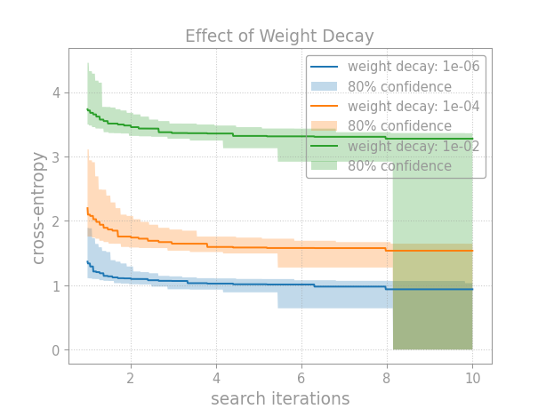
Breaking down this example, first we choose values at which to probe the hyperparameter:

>>> weight_decays = [1e-6, 1e-4, 1e-2]

Then, we fix the hyperparameter to each value (1e-6, 1e-4, 1e-2) in a separate random search:

>>> conditions = []
>>> for weight_decay in weight_decays:
...   name = f"weight decay: {weight_decay:.0e}"
...   ys = pretrain(
...     learning_rate=np.exp(uniform(np.log(1e-5), np.log(1e-1), size=n)),
...     weight_decay=weight_decay,
...   )
...   conditions.append((name, ys))

After collecting the results, we construct confidence bands:

>>> for name, ys in conditions:
...   # Construct the confidence bands.
...   dist_lo, dist_pt, dist_hi = EmpiricalDistribution.confidence_bands(
...     ys=ys,            # cross-entropy results from random search
...     confidence=0.80,  # confidence level
...     a=0.,             # (optional) lower bound on cross-entropy
...     b=np.inf,         # (optional) upper bound on cross-entropy
...   )

And then plot the tuning curves:

...   # Plot the tuning curve.
...   ax.plot(
...     ns,
...     dist_pt.quantile_tuning_curve(ns, minimize=True),
...     label=name,
...   )
...   # Plot the confidence bands.
...   ax.fill_between(
...     ns,
...     dist_hi.quantile_tuning_curve(ns, minimize=True),
...     dist_lo.quantile_tuning_curve(ns, minimize=True),
...     alpha=0.275,
...     label="80% confidence",
...   )

Last, we just format the plots then save or show them.

For more information, checkout EmpiricalDistribution in the reference documentation or get interactive help in a Python REPL by running help(EmpiricalDistribution).

Footnotes

[1]

For a great example calculating these kinds of quantities for a transformer, see Section 2 of Scaling Laws for Neural Language Models (Kaplan et al., 2020).