Usage#

Opda helps you compare machine learning methods while accounting for their hyperparameters. This guide reviews opda’s basic functionality, while Examples walks through how to run such an analysis.

Working with the Empirical Distribution#

Many analyses in opda are designed around random search. Each round of random search independently samples a choice of hyperparameters and then evaluates it, producing a score (like accuracy). The probability distribution over these scores determines how good the model is, and how quickly performance goes up with more hyperparameter tuning effort. Given a bunch of scores from random search, you can estimate this distribution with the empirical distribution of the sample.

If ys is an array of scores from random search, you can represent the empirical distribution with the EmpiricalDistribution class:

>>> from opda.nonparametric import EmpiricalDistribution
>>> import opda.random
>>>
>>> opda.random.set_seed(0)
>>>
>>> dist = EmpiricalDistribution(
...   ys=[.72, .83, .92, .68, .75],  # scores from random search
...   ws=None,                       # (optional) sample weights
...   a=0.,                          # (optional) lower bound on the score
...   b=1.,                          # (optional) upper bound on the score
... )

Using the class, you can do many things you might expect with a probability distribution. For example, you can sample from it:

>>> dist.sample()
0.75
>>> dist.sample(2)
array([0.68, 0.92])
>>> dist.sample(size=(2, 3))
array([[0.83, 0.83, 0.72],
       [0.72, 0.72, 0.72]])

You can compute the PMF (probability mass function):

>>> dist.pmf(0.5)
0.0
>>> dist.pmf(0.75)
0.2
>>> dist.pmf([0.5, 0.75])
array([0. , 0.2])

the CDF (cumulative distribution function):

>>> dist.cdf(0.5)
0.0
>>> dist.cdf(0.72)
0.4
>>> dist.cdf([0.5, 0.72])
array([0. , 0.4])

and even the quantile function, also known as the percentile-point function or PPF:

>>> dist.ppf(0.0)
0.0
>>> dist.ppf(0.4)
0.72
>>> dist.ppf([0.0, 0.4])
array([0.  , 0.72])

The EmpiricalDistribution class also prints nicely and supports equality checks:

>>> EmpiricalDistribution(ys=[0.5, 1.], a=-1., b=1.)
EmpiricalDistribution(ys=array([0.5, 1. ]), ws=None, a=-1.0, b=1.0)
>>> EmpiricalDistribution([1.]) == EmpiricalDistribution([1.])
True

Estimating Tuning Curves#

EmpiricalDistribution provides several methods for estimating tuning curves. Tuning curves plot the median score as a function of hyperparameter tuning effort. Thus, tuning curves capture the cost-benefit trade-off offered by tuning a model’s hyperparameters.

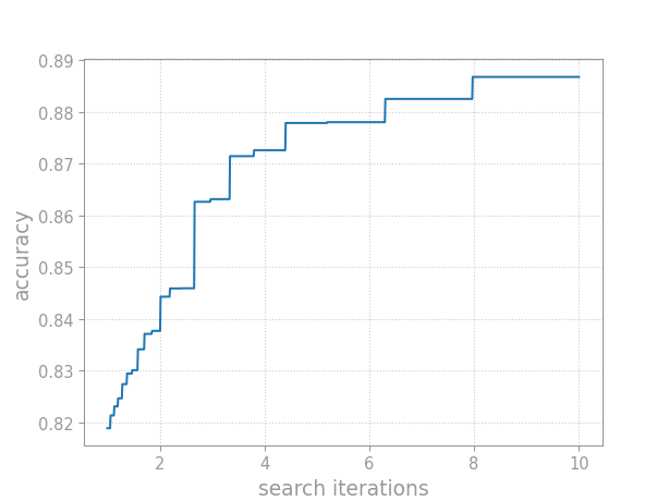
../_images/usage-1.png — The median tuning curve plots the score as a function of tuning effort.#

You can compute the median tuning curve using quantile_tuning_curve():

>>> dist.quantile_tuning_curve(1)
0.75
>>> dist.quantile_tuning_curve([1, 2, 4])
array([0.75, 0.83, 0.92])

quantile_tuning_curve() computes the median tuning curve by default, but you can also explicitly pass the q argument to compute the 20th, 95th, or any other quantile of the tuning curve:

>>> dist.quantile_tuning_curve([1, 2, 4], q=0.2)
array([0.68, 0.75, 0.83])

In this way, you can describe the entire distribution of scores from successive rounds of random search.

Depending on your metric, you may want to minimize a loss rather than maximize a utility. Control minimization versus maximization using the minimize argument:

>>> dist.quantile_tuning_curve([1, 2, 4], minimize=True)
array([0.75, 0.72, 0.68])

While the median tuning curve is recommended, you can also compute the expected tuning curve with average_tuning_curve():

>>> dist.average_tuning_curve([1, 2, 4])
array([0.78    , 0.8272  , 0.871936])

Constructing Confidence Bands#

In theory, tuning curves answer any question you might ask about performance as a function of tuning effort. In practice, tuning curves must be estimated from data. Thus, we need to know how reliable such estimates are. Confidence bands quantify an estimate’s reliability.

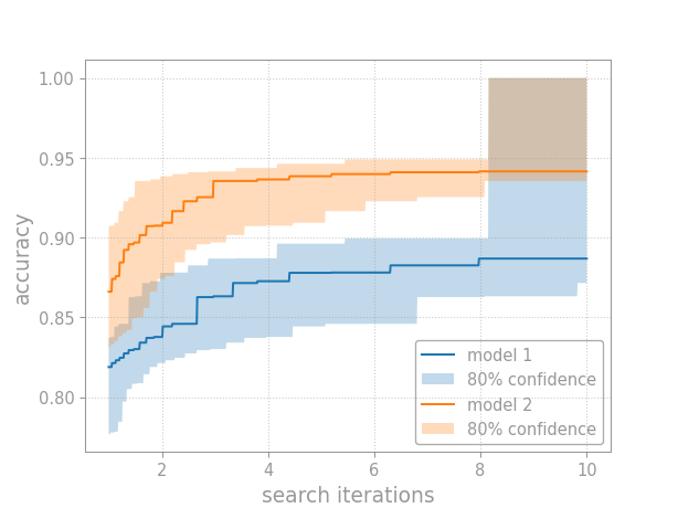
../_images/usage-2.png — Confidence bands quantify uncertainty when comparing models.#

Opda offers simultaneous confidence bands that contain the entire curve at once. You can compute simultaneous confidence bands for the CDF and then translate these to the tuning curve.

Cumulative Distribution Functions#

Compute simultaneous confidence bands for the CDF using the confidence_bands() class method:

>>> dist_lo, dist_pt, dist_hi = EmpiricalDistribution.confidence_bands(
...   ys=[.72, .83, .92, .68, .75],  # scores from random search
...   confidence=0.80,               # the confidence level
...   a=0.,                          # (optional) lower bound on the score
...   b=1.,                          # (optional) upper bound on the score
... )

The returned objects, dist_lo, dist_pt, and dist_hi, are EmpiricalDistribution instances respectively representing the lower band, point estimate, and upper band for the empirical distribution.

Thus, you can use dist_pt to estimate the CDF:

>>> dist_pt == EmpiricalDistribution([.72, .83, .92, .68, .75], a=0., b=1.)
True
>>> dist_pt.cdf([0., 0.72, 1.])
array([0. , 0.4, 1. ])

While dist_lo and dist_hi bound the CDF:

>>> all(dist_lo.cdf([0., 0.72, 1.]) <= dist_pt.cdf([0., 0.72, 1.]))
True
>>> all(dist_pt.cdf([0., 0.72, 1.]) <= dist_hi.cdf([0., 0.72, 1.]))
True

The bounds from confidence_bands() are guaranteed to contain the true CDF with probability equal to confidence, as long as the underlying distribution is continuous and the scores are independent.

Tuning Curves#

When comparing models, we don’t care primarily about the CDF but rather the tuning curve. Given confidence bounds on the CDF, we can easily convert these into bounds on the tuning curve using the quantile_tuning_curve() method. In particular, the lower CDF bound gives the upper tuning curve bound, and the upper CDF bound gives the lower tuning curve bound:

>>> ns = range(1, 11)
>>> tuning_curve_lo = dist_hi.quantile_tuning_curve(ns)
>>> tuning_curve_pt = dist_pt.quantile_tuning_curve(ns)
>>> tuning_curve_hi = dist_lo.quantile_tuning_curve(ns)
>>>
>>> all(tuning_curve_lo <= tuning_curve_pt)
True
>>> all(tuning_curve_pt <= tuning_curve_hi)
True

This reversal occurs because the CDF maps from the scores (e.g., accuracy numbers), while the tuning curve maps to the scores. Swapping the direction of the mapping also swaps the inequalities on the bounds.

Running the notebooks#

Several notebooks are available in opda’s source repository. These notebooks offer experiments and develop the theory behind opda.

To run the notebooks, make sure you’ve installed the necessary optional dependencies. Then, run the notebook server:

$ cd nbs/ && jupyter notebook

And open up the URL printed to the console.

Getting More Help#

More documentation is available for exploring opda even further.

Interactive Help#

Opda is self-documenting. Use help() to view the documentation for a function or class in the REPL:

>>> from opda.nonparametric import EmpiricalDistribution
>>> help(EmpiricalDistribution)  
Help on class EmpiricalDistribution in module opda.nonparametric:

class EmpiricalDistribution(builtins.object)
 |  EmpiricalDistribution(ys, ws=None, a=-inf, b=inf)
 |
 |  The empirical distribution.
 |
 |  Parameters
 |  ----------
 |  ys : 1D array of floats, required
 |      The sample for which to create an empirical distribution.
...

Interactive shell and REPL sessions are a great way to explore opda!

API Reference#

The API Reference documents every aspect of opda.

The parametric and nonparametric modules implement much of the core functionality.